[comm] MIMO Shannon Capacity: From Scalars to Matricies

0. Introduction: Why MIMO?

In the previous post, we observed that the SISO capacity increases only logarithmically with transmit power ($P_{tx}$). This logarithmic growth represents a physical wall; doubling the power does not double the data rate.

To overcome this, MIMO (Multiple-Input Multiple-Output) systems utilize the spatial domain. By using multiple antennas at both the transmitter and receiver, we can create multiple parallel “pipes” in the same frequency band, achieving a linear increase in capacity with the number of antennas.

In this post, we will transition from scalar models to vector/matrix models and derive the MIMO capacity formula.

---

1. System Model: Multi-user MIMO (BC)

To analyze the capacity and beamforming strategies in a modern network, we transition from a point-to-point link to a Multi-user MIMO (MU-MIMO) scenario, specifically the Broadcast Channel (BC). The model describes a Base Station (BS) communicating with multiple User Equipments (UEs) simultaneously.

The received signal for the $k$-th user is modeled as:

\[\mathbf{y}_k = \mathbf{H}_k \mathbf{x} + \mathbf{n}_k\]

Key Parameters:

• $P$ (Transmit Antennas): The number of antennas at the Base Station (Transmitter).
• $Q$ (Receive Antennas): The number of antennas at each User Equipment (Receiver). For simplicity, we often assume each user has the same number of antennas $Q$.
• $K$ (Total Users): The number of independent users being served by the Base Station in the same time-frequency resource.
• $\mathbf{x} \in \mathbb{C}^{P \times 1}$: The aggregate transmitted signal vector from the Base Station.
• $\mathbf{y}_k \in \mathbb{C}^{Q \times 1}$: The signal received by the $k$-th user.
• $\mathbf{H}_k \in \mathbb{C}^{Q \times P}$: The channel matrix between the BS and the $k$-th user.
• $\mathbf{n}_k \sim \mathcal{CN}(0, \sigma_n^2 \mathbf{I}_Q)$: The Additive White Gaussian Noise (AWGN) at the $k$-th user’s receiver.

Transmit Autocorrelation and Power Constraint

In this multi-user context, the transmitted signal $\mathbf{x}$ is typically a combination of independent data streams intended for each of the $K$ users. To characterize the spatial properties and power distribution of the aggregate signal, we define the Input Autocorrelation Matrix $\mathbf{R}_{xx}$:

\[\mathbf{R}_{xx} = \mathbb{E}[\mathbf{xx}^\text{H}] \in \mathbb{C}^{P \times P}\]

The total transmit power budget $P_$ at the Base Station must be shared among all $K$ users. This physical limitation is expressed via the Trace of the autocorrelation matrix:

\[\text{Tr}(\mathbf{R}_{xx}) \le P_\]

In a Broadcast Channel, the Base Station must design the precoding (beamforming) strategy within $\mathbf{x}$ to maximize the sum-rate while managing the Inter-User Interference (IUI). This leads directly to the need for advanced optimization frameworks like the WMMSE algorithm to handle the resulting non-convex problems.

---

3. Derivation of Achievable Rate $R_k$ in MU-MIMO

Following the multivariate entropy results, we can now derive the achievable rate for each user in a Multi-user MIMO (MU-MIMO) Broadcast Channel. We assume the Base Station (BS) uses transmit filters (beamformers) $\mathbf{B}_k \in \mathbb{C}^{P \times Q}$ for each user $k \in {1, \dots, K}$.

3.1 Signal Model with Beamforming

The aggregate transmitted signal $\mathbf{x}$ is the sum of signals intended for all $K$ users: \(\mathbf{x} = \sum_{k=1}^K \mathbf{B}_k \mathbf{d}_k\) where $\mathbf{d}_k \sim \mathcal{CN}(0, \mathbf{I}_Q)$ is the data vector for user $k$. The received signal at user $k$ is: \(\mathbf{y}_k = \mathbf{H}_k \mathbf{B}_k \mathbf{d}_k + \sum_{j \neq k}^K \mathbf{H}_k \mathbf{B}_j \mathbf{d}_j + \mathbf{n}_k\) To simplify the derivation, we define the Interference-plus-Noise term as $\tilde{\mathbf{v}}_k$: \(\tilde{\mathbf{v}}_k = \sum_{j \neq k}^K \mathbf{H}_k \mathbf{B}_j \mathbf{d}_j + \mathbf{n}_k\)

3.2 Information Theoretic Derivation

The achievable rate $R_k$ is the maximum mutual information between the sent data $\mathbf{d}_k$ and the received signal $\mathbf{y}_k$:

\[\begin{aligned} R_k &= I(\mathbf{d}_k ; \mathbf{y}_k) \\ &= H(\mathbf{y}_k) - H(\mathbf{y}_k | \mathbf{d}_k) \\ &= H(\mathbf{y}_k) - H(\tilde{\mathbf{v}}_k) \end{aligned}\]

Using our previously derived result for multivariate complex Gaussian entropy, $H(\mathbf{x}) = \log_2 \det(\pi e \mathbf{R}_{xx})$, we can write:

\[R_k = \log_2 \det(\pi e \mathbf{R}_{y_k y_k}) - \log_2 \det(\pi e \mathbf{R}_{\tilde{v}_k \tilde{v}_k})\]

Applying the property $\log \det(\mathbf{A}) - \log \det(\mathbf{B}) = \log \det(\mathbf{A} \mathbf{B}^{-1})$, the formula simplifies to:

\[R_k = \log_2 \det \left( \mathbf{R}_{y_k y_k} \mathbf{R}_{\tilde{v}_k \tilde{v}_k}^{-1} \right)\]

3.3 Autocorrelation Matrix Expansion

To reach the final engineering formula, we expand the autocorrelation matrices $\mathbf{R}{y_k y_k}$ and $\mathbf{R}{\tilde{v}_k \tilde{v}_k}$. Assuming data and noise are independent and zero-mean:

1. Interference plus Noise Covariance: \(\mathbf{R}_{\tilde{v}_k \tilde{v}_k} = \mathbb{E}[\tilde{\mathbf{v}}_k \tilde{\mathbf{v}}_k^{\text{H}}] = \sum_{j \neq k}^K \mathbf{H}_k \mathbf{B}_j \mathbf{B}_j^{\text{H}} \mathbf{H}_k^{\text{H}} + \sigma_n^2 \mathbf{I}_Q\)

2. Received Signal Covariance: \(\mathbf{R}_{y_k y_k} = \mathbb{E}[\mathbf{y}_k \mathbf{y}_k^{\text{H}}] = \mathbf{H}_k \mathbf{B}_k \mathbf{B}_k^{\text{H}} \mathbf{H}_k^{\text{H}} + \mathbf{R}_{\tilde{v}_k \tilde{v}_k}\)

Substituting these back into the rate equation and using the identity $\det(\mathbf{I} + \mathbf{AB}) = \det(\mathbf{I} + \mathbf{BA})$, we obtain the standard MU-MIMO achievable rate formula:

\[R_k = \log_2 \det \left( \mathbf{I}_Q + \mathbf{H}_k \mathbf{B}_k \mathbf{B}_k^{\text{H}} \mathbf{H}_k^{\text{H}} \mathbf{R}_{\tilde{v}_k \tilde{v}_k}^{-1} \right)\]

3.4 Applying Sylvester’s Determinant Identity

In many optimization frameworks like WMMSE, it is more convenient to express the rate in terms of the transmit filter dimensions. We use the identity $\det(\mathbf{I}_m + \mathbf{AB}) = \det(\mathbf{I}_n + \mathbf{BA})$ to swap the order of the matrices.

By setting $\mathbf{A} = \mathbf{H}k \mathbf{B}_k$ and $\mathbf{B} = \mathbf{B}_k^{\text{H}} \mathbf{H}_k^{\text{H}} \mathbf{R}{\tilde{v}_k \tilde{v}_k}^{-1}$, we can rewrite the rate for user $k$ as:

\[R_k = \log_2 \det \left( \mathbf{I}_k + \mathbf{B}_k^{\text{H}} \mathbf{H}_k^{\text{H}} \mathbf{R}_{\tilde{v}_k \tilde{v}_k}^{-1} \mathbf{H}_k \mathbf{B}_k \right), \tag{5}\]

Here, $\mathbf{I}_k$ represents the identity matrix corresponding to the number of data streams (or receive antennas $Q$) for user $k$. This specific form is the cornerstone of the WMMSE algorithm, as the term inside the determinant is directly related to the inverse of the Error Covariance matrix.

Summary of Dimensions

• Transmit Signal: $\mathbf{x} \in \mathbb{C}^{P \times 1}$
• Beamforming Matrix: $\mathbf{B}_k \in \mathbb{C}^{P \times Q}$
• Channel Matrix: $\mathbf{H}_k \in \mathbb{C}^{Q \times P}$
• Total Transmit Power: $\text{Tr}(\sum_{k=1}^K \mathbf{B}k \mathbf{B}_k^{\text{H}}) \le P{\text{tx}}$

---

4. Analysis and Simulation

To verify the theoretical gains of moving from a single antenna to a multi-user MIMO system, we can simulate the sum capacity across various signal-to-noise ratios (SNR). This simulation allows us to visualize how increasing the number of antennas and users impacts the overall data rate of the system.

4.1 Python Implementation: SISO vs. MIMO Comparison

The following script calculates the sum rate based on the system model where a Base Station (BS) with $P$ antennas serves $K$ users, each equipped with $Q$ antennas. For this baseline simulation, we assume uniform power allocation across the transmit antennas.

import numpy as np
import matplotlib.pyplot as plt

def calculate_mimo_capacity(snr_db, p, q, k=1):
    """
    Calculates sum capacity for MU-MIMO (BC) with uniform power allocation.
    P: Transmit Antennas (BS)
    Q: Receive Antennas (UE)
    K: Number of Users
    """
    snr_lin = 10**(snr_db / 10.0)
    
    # Total power is shared among all users (uniform allocation)
    # Power per user stream
    power_per_user = snr_lin / k 
    
    total_sum_rate = 0
    for _ in range(k):
        # Generate i.i.d. Rayleigh Fading Channel H_k (Q x P)
        H_k = (np.random.randn(q, p) + 1j * np.random.randn(q, p)) / np.sqrt(2)
        
        # Using Equation (5) logic for a single user rate:
        # R_k = log2 det(I + (SNR/P) * H * H^H) 
        # Here we assume Rx = (P_tx / P) * I (Uniform power per antenna)
        core_matrix = np.eye(q) + (snr_lin / p) * (H_k @ H_k.conj().T)
        total_sum_rate += np.real(np.log2(np.linalg.det(core_matrix)))
        
    return total_sum_rate

# Simulation Parameters
snr_range = np.linspace(-10, 40, 20)
configs = [
    {'label': 'SISO (P=1, Q=1, K=1)', 'p': 1, 'q': 1, 'k': 1},
    {'label': 'MIMO (P=2, Q=2, K=1)', 'p': 2, 'q': 2, 'k': 1},
    {'label': 'MIMO (P=4, Q=4, K=1)', 'p': 4, 'q': 4, 'k': 1},
    {'label': 'MU-MIMO (P=8, Q=2, K=4)', 'p': 8, 'q': 2, 'k': 4}
]

plt.figure(figsize=(10, 7))

for config in configs:
    # Averaging over multiple channel realizations for a smooth curve
    capacity_results = []
    for snr in snr_range:
        avg_cap = np.mean([calculate_mimo_capacity(snr, config['p'], config['q'], config['k']) for _ in range(50)])
        capacity_results.append(avg_cap)
    
    plt.plot(snr_range, capacity_results, label=config['label'], marker='o', markersize=4)

plt.title('Spectral Efficiency Comparison: SISO vs. MIMO Variants', fontsize=14)
plt.xlabel('SNR (dB)', fontsize=12)
plt.ylabel('Sum Capacity (bits/s/Hz)', fontsize=12)
plt.grid(True, linestyle='--', alpha=0.7)
plt.legend()
plt.show()

4.2 Results Interpretation

The simulation results clearly demonstrate the performance gap between different antenna configurations:

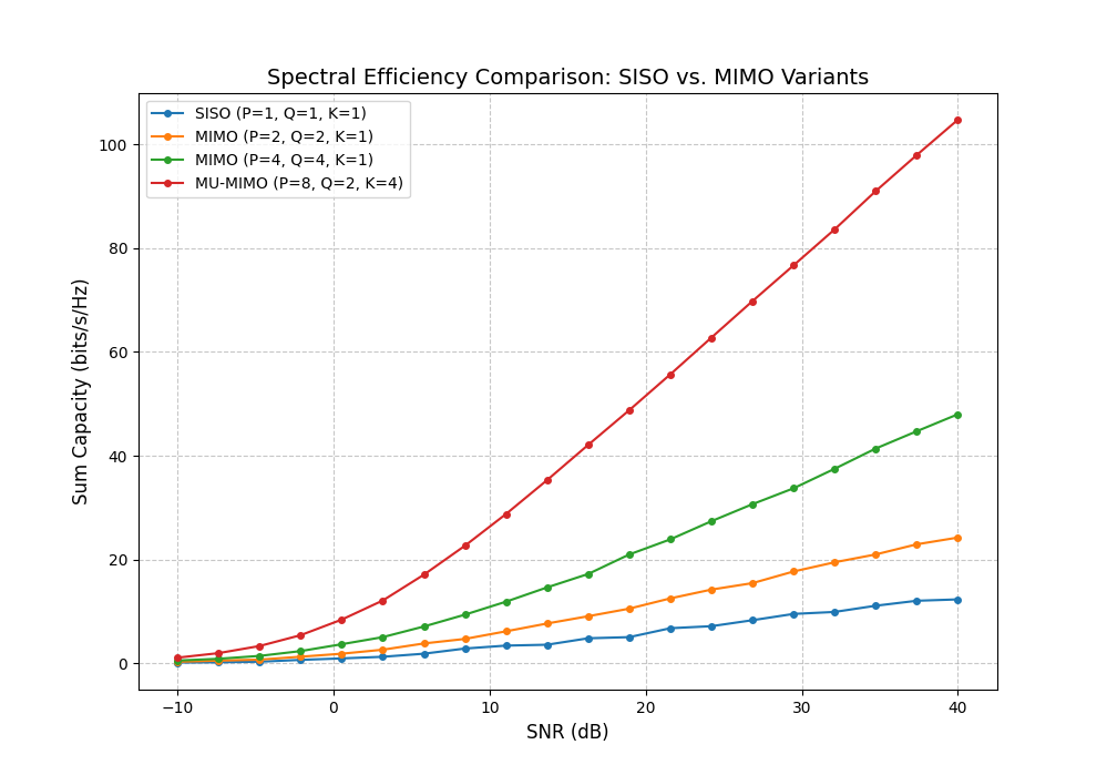
• SISO Baseline: The curve for $P=1, Q=1$ shows the slowest growth, as it is limited to a single spatial channel.
• MIMO Advantage: As we increase the number of antennas at both ends ($2 \times 2$ and $4 \times 4$), the capacity grows much faster with SNR. This is because the system can exploit multiple spatial paths created by the channel matrix $\mathbf{H}$.
• Multi-user MIMO Performance: The MU-MIMO (P=8, Q=2, K=4) configuration achieves the highest sum capacity. By serving multiple users ($K=4$) simultaneously using a large antenna array at the Base Station ($P=8$), the system significantly multiplies the total data rate compared to single-user scenarios.
• The Need for Optimization: While these results show significant gains even with uniform power, they represent a simplified case. In real-world environments with inter-user interference, we need more sophisticated beamforming strategies—like the WMMSE algorithm—to maximize these rates by precisely shaping the transmit filters $\mathbf{B}_k$.

---

5. Conclusion

Through this exploration, we have transitioned from the fundamental SISO Shannon capacity to the complex, multi-dimensional world of MU-MIMO. The simulation results confirm that leveraging the spatial domain through multiple antennas is the most effective way to overcome the logarithmic limitations of traditional wireless links.

However, achieving these gains in a real-world multi-user environment requires more than just adding antennas; it requires precise control over signal interference. This leads us to the necessity of advanced optimization frameworks.

---

References

• Christensen, Søren Skovgaard, et al. “Weighted Sum-Rate Maximization Using Weighted MMSE for MIMO-BC Beamforming Design.” IEEE Transactions on Wireless Communications, vol. 7, no. 12, Dec. 2008, pp. 4792–99. DOI.org (Crossref), https://doi.org/10.1109/T-WC.2008.070851.