[comm] SISO Shannon Capacity: Deriving the Rate Limit via Entropy

0. Intro: The Physical Limit of Throughput

In communication systems, is there a theoretical upper bound on the amount of information that can be transmitted over a physical channel?

In his seminal 1948 paper, Claude Shannon proved that such a limit exists, now known as the Channel Capacity. This limit is determined not only by the technology used but by the fundamental physics of signal power, noise, and bandwidth.

This post explores the derivation of the SISO (Single-Input Single-Output) capacity formula from the perspective of Information Theory. Understanding this derivation is crucial for extending these concepts to MIMO (Multiple-Input Multiple-Output) systems and advanced optimization algorithms like WMMSE.

1. System Model

Consider a point-to-point communication channel modeled as:

\[y = hx + n\]

• $x$: Transmitted complex symbol.
• $y$: Received signal.
• $h$: Channel coefficient. For this derivation, we assume a static channel gain normalized to $\left\vert{h}\right\vert =1$.
• $n$: Additive White Gaussian Noise (AWGN) with variance $\sigma_n^2$.

Physical Constraints

Any practical system operates under two primary constraints:

1. Average Power Constraint: The transmitter has a limited power budget $P_{tx}$. \(\mathbb{E}[|x|^2] \le P_{tx}\)
2. Bandwidth Constraint: The system is band-limited to $B$ Hz.

2. Entropy: The Measure of Uncertainty

To understand the limit of data transmission, we must first quantify “information.” In Information Theory, Entropy measures the average uncertainty or “surprise” of a random variable.

2.1 Definition

If an event is highly probable, it contains little information (no surprise). If an event is rare, it carries high information.

For a discrete random variable $X$, the Shannon Entropy $H(X)$ is defined as:

\[H(X) = - \sum_{i} p(x_i) \log_2 p(x_i)\]

However, physical signals (voltage, current) are continuous. For continuous random variables, we use Differential Entropy:

\[h(x) = - \int_{-\infty}^{\infty} f(x) \log_2 f(x) dx\]

• $f(x)$: Probability Density Function (PDF)
• Unlike discrete entropy, differential entropy can be negative, but it still serves as a relative measure of randomness.

2.2 Why Gaussian?

In communication systems, we specifically focus on the Gaussian distribution. Why?

There is a fundamental theorem in information theory:

“For a given variance (average power constraints), the distribution that maximizes differential entropy is the Gaussian distribution.”

Since we want to maximize the information transfer (Capacity) under a limited power budget ($P_{tx}$), we assume the signal $x$ follows a Complex Normal distribution:

\[H(\mathcal{CN}) = \log_2(\pi e \sigma^2)\]

For a detailed step-by-step derivation of why Gaussian entropy results in log(πeσ2), you can check it here

This simple logarithmic relation between “Power ($\sigma^2$)” and “Information ($H$)” is the key to deriving the channel capacity.

3. Derivation of Shannon Capacity

Now, let’s derive the capacity formula. The achievable rate $R$ is defined by the Mutual Information $I(X; Y)$ between the transmitted signal $X$ and the received signal $Y$

Intuitively, the rate is the total information received minus the useless information (uncertainty) introduced by noise.

\[R = I(X; Y) = H(Y) - H(Y|X)\]

Step 1: Breakdown

Since $Y = X + N$, if we know $X$, the only uncertainty remaining in $Y$ is the noise $N$.
Thus, $H(Y|X) = H(N)$

\[R = H(Y) - H(N)\]

This equation essentially says: “The net information is the entropy of the received signal minus the entropy of the noise.”

Step 2: Applying Gaussian Entropy

Using the formula for Gaussian entropy derived above:

1. Received Signal ($Y$): The power of $Y$ is the sum of signal power ($S$) and noise power ($N$). \(\sigma_y^2 = S + N\) \(H(Y) = \log_2(\pi e (S + N))\)

2. Noise ($N$): \(\sigma_n^2 = N\) \(H(N) = \log_2(\pi e N)\)

Step 3: The Result

Substitute these back into the rate equation:

\[\begin{aligned} R &= \log_2(\pi e (S + N)) - \log_2(\pi e N) \\ &= \log_2 \left( \frac{\pi e (S + N)}{\pi e N} \right) \\ &= \log_2 \left( \frac{S + N}{N} \right) \\ &= \log_2 \left( 1 + \frac{S}{N} \right) \quad (\text{bits/s/Hz}) \end{aligned}\]

Finally, multiplying by the available bandwidth $B$ gives the famous Shannon Capacity formula:

\[C = B \log_2 \left( 1 + \text{SNR} \right) \quad (\text{bps})\]

4. Analysis and Simulation

The formula reveals two distinct regimes for increasing capacity:

1. Bandwidth Limited Regime: Capacity increases linearly with bandwidth $B$.
2. Power Limited Regime: Capacity increases logarithmically with SNR. Due to the $\log$ function, increasing transmit power yields diminishing returns in terms of data rate.

Numerical Verification

The following Python script simulates the relationship between SNR and Spectral Efficiency.

import numpy as np
import matplotlib.pyplot as plt

def calculate_capacity(snr_db):
    """
    Computes Spectral Efficiency (bits/s/Hz) given SNR in dB.
    Formula: C = log2(1 + SNR_linear)
    """
    # Convert dB to Linear scale
    snr_linear = 10 ** (snr_db / 10.0)
    
    # Calculate Capacity (assuming normalized bandwidth B=1)
    capacity = np.log2(1 + snr_linear)
    return capacity

# 1. Simulation Parameters
snr_db_range = np.linspace(-10, 40, 100) # SNR range: -10dB to 40dB

# 2. Compute Capacity
capacities = calculate_capacity(snr_db_range)

# 3. Visualization
plt.figure(figsize=(10, 6))
plt.plot(snr_db_range, capacities, label='Shannon Capacity Limit', linewidth=2)

plt.title('Spectral Efficiency vs. SNR', fontsize=16)
plt.xlabel('SNR (dB)', fontsize=14)
plt.ylabel('Spectral Efficiency (bits/s/Hz)', fontsize=14)
plt.grid(True, which="both", ls="--", alpha=0.6)
plt.legend()
plt.tight_layout()
plt.show()

Observation

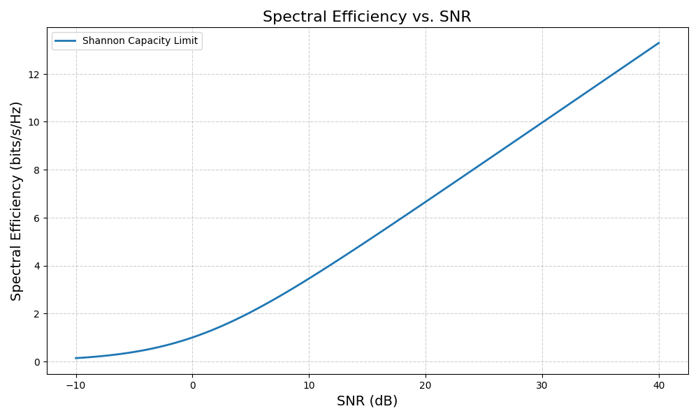
Note that the y-axis of the plot is shown on a logarithmic scale.

The plot demonstrates the logarithmic nature of capacity with respect to power. To achieve a linear increase in data rate, the power must be increased exponentially. This physical limitation necessitates the use of spatial multiplexing techniques (MIMO) to overcome the single-channel capacity barrier.

5. Conclusion & Next Steps

We have derived the SISO capacity limit using the concept of Differential Entropy. The key takeaway is that capacity is fundamentally a measure of the “volume” of the signal space relative to the noise space.

In the next post, I will extend this derivation to MIMO (Multiple-Input Multiple-Output) systems. We will observe how the scalar variance transforms into a Covariance Matrix, and how the simple logarithm evolves into the Log-Determinant ($\log$ $\det$), a crucial component in modern beamforming optimization.

---

References

• Christensen, Søren Skovgaard, et al. “Weighted Sum-Rate Maximization Using Weighted MMSE for MIMO-BC Beamforming Design.” IEEE Transactions on Wireless Communications, vol. 7, no. 12, Dec. 2008, pp. 4792–99. DOI.org (Crossref), https://doi.org/10.1109/T-WC.2008.070851.